| Day | Concept | Key Learning |
|---|---|---|
| 1 | Sin & Cos Waves | Oscillation / Cycles |
| 2 | Brownian Motion | Random motion |
| 3 | Perlin Noise | Smooth randomness |
| 4 | Fractal Brownian Motion (fBm) | Layered complexity |
| 5 | Mass-Spring Systems | Force, bounce, interactivity |
The next step was creating the lesson sketches, which took up the largest portion of time. I carefully ensured all the materials were well-aligned, and included necessary explanations so the content would be easy to teach and understand. These would be edited and changed as I got feedback so they are understood as best they can be. I removed lesson 6 from the plan due to time issues, but they will soon be added in once completed.
The sketches made for the lessons are here:
https://editor.p5js.org/arajkumar/collections/Dv4yNVvXx
Here, I also documented how I might want to approach my lesson in terms of teaching – experimenting with my own example, or building it from scratch in the class, while teaching to demonstrate the concepts, and prompts to expand and link it to animation. This, too, may have varied during the actual delivery of the lesson and may change when it is put onto the website after they are delivered and feedback has been implemented, but it provides a rough structure.
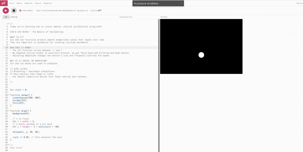
Objective:
To understand and visualise smooth oscillating motion using sine and cosine functions, useful for natural & rhythmic animations.
Concept Overview:
Sine and cosine functions generate smooth, periodic oscillations, which can be mapped to position / rotation to create natural, repeating movements. These functions cycle between -1 and 1 continuously, allowing for a fluid back-and-forth or up-and-down motion.
Step-by-Step Approach:
- Set up the canvas: Create a simple black-and-white environment for clear visualisation.
- Define animation parameters: Initialise variables to control amplitude (motion size), frequency (speed), and phase (starting position).
- Calculate position: Use
sin()orcos()functions with a time variable (usually frame count or elapsed time) to compute the oscillating value. - Map sine output: Scale the sine output to the desired range on the screen, e.g., vertical or horizontal movement limits.
- Draw the object: Render a shape (like a circle) at the calculated position to visualise the oscillation.
- Animate over time: Increment the time variable continuously to produce ongoing smooth motion.
Animation Applications:
- Breathing effects
- Walk cycles (limb oscillations)
- Any repetitive, rhythmic motion that requires smooth transitions
Tips for Experimentation:
- Vary amplitude to change motion size.
- Adjust frequency to speed up or slow down oscillations.
- Combine sine and cosine for complex paths or phase shifts.
- Layer multiple waves for more natural or complex effects.
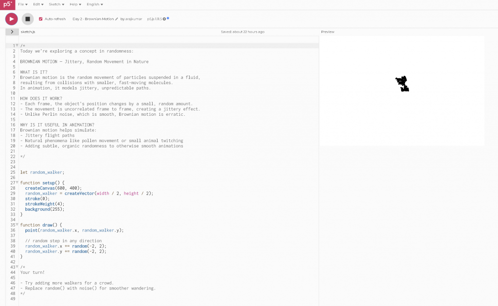
Objective:
To simulate natural, random, jittery movement to create organic, unpredictable animation effects.
Concept Overview:
Brownian motion models the random motion of particles suspended in fluid, resulting in erratic and jittery paths. In animation, it’s a simple but powerful technique to simulate unpredictable, organic movement.
Step-by-Step Approach:
- Set up the canvas: Use a black-and-white scheme to focus on movement clarity.
- Initialise position: Start with an object at a fixed or random position.
- Apply random movement: Each frame, add a small random offset to the object’s position (both x and y).
- Update continuously: Animate by updating the position every frame, producing a “drunken walk” effect.
Animation Applications:
- Dust particles drifting in the air
- Small animals or insects jittery movement
- Leaf fluttering
Tips for Experimentation:
- Adjust size of the random offset to control jitteriness intensity.
- Combine Brownian motion with other motion types for more complex behavior.
- Use Brownian motion to add subtle natural variation to otherwise smooth animations.
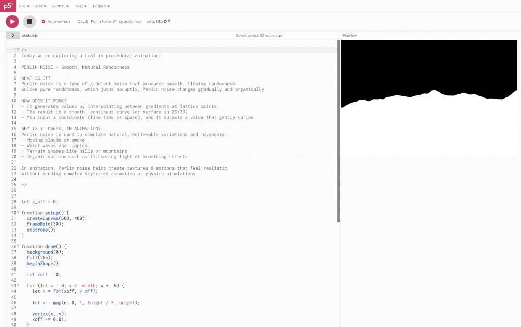
Objective:
To generate smooth, flowing randomness for natural motion and organic shapes in animation.
Concept Overview:
Perlin noise produces coherent & smooth random values that vary gradually over space or time. Unlike pure random noise, Perlin noise avoids harsh jumps, creating fluid transitions ideal for natural effects.
Step-by-Step Approach:
- Set up the canvas: Black-and-white style for easy observation of smooth changes.
- Define input variable: Use time or spatial coordinates as input to the noise function.
- Sample noise: Call
noise()with the input variable to get a smooth value between 0 and 1. - Map output: Scale the noise output to desired position, color, or shape ranges.
- Animate: Increment input variable over time for continuous, smooth changes.
Animation Applications:
- Flowing water or smoke
- Cloud and fog textures
- Natural terrain shapes like mountains or waves
Tips for Experimentation:
- Use multiple dimensions of noise (1D, 2D, or 3D) for more complex animations.
- Combine Perlin noise with oscillation for richer motion patterns.
- Adjust the speed of input changes to control smoothness and speed.
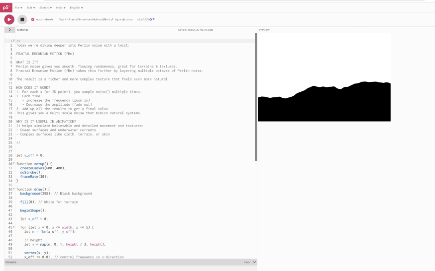
Objective:
To create complex, detailed organic motion and textures by layering multiple octaves of Perlin noise.
Concept Overview:
Fractal Brownian Motion (fBm) layers several frequencies of Perlin noise, each with different amplitudes, to create richer and more natural-looking patterns. Think of it as combining big smooth waves with smaller ripples and tiny vibrations.
Step-by-Step Approach:
- Set up the canvas: Keep it black and white for contrast.
- Define noise layers: Sample Perlin noise at increasing frequencies (zooming in).
- Weight layers: Apply decreasing amplitude to higher-frequency noise layers.
- Sum layers: Combine weighted noise values for final output.
- Animate: Increment base input over time for evolving, detailed motion.
Animation Applications:
- Realistic ocean waves with texture
- Wind-blown grass or hair detail
- Wrinkled fabric or skin textures
- Atmospheric effects like clouds and fog
Tips for Experimentation:
- Adjust number of octaves and weights for different detail levels.
- Mix with color or shape changes for richer effects.
- Use as a base for procedural textures or terrains.
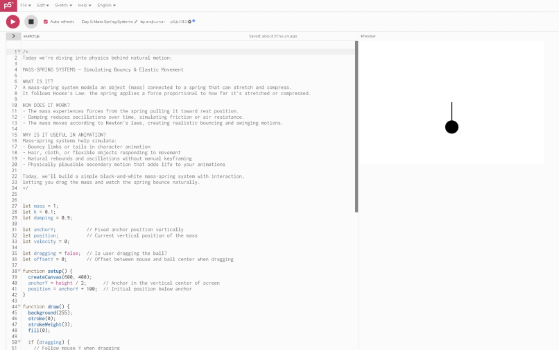
Objective:
To simulate realistic bouncy and elastic motion using physics-based spring and damping models.
Concept Overview:
A mass-spring system models objects connected to springs that exert restoring forces. When displaced, the system oscillates and gradually comes to rest due to damping, simulating realistic movement of limbs, hair, or soft materials.
Step-by-Step Approach:
- Set up canvas: Black-and-white for clarity.
- Initialise mass position, velocity, and acceleration.
- Define spring parameters: Rest length, spring constant, and damping factor.
- Calculate spring force: Apply Hooke’s law based on displacement from rest.
- Update physics: Compute acceleration from force, update velocity and position.
- Animate: Repeat physics update each frame for smooth spring motion.
Animation Applications:
- Bouncy limbs in walk or run cycles
- Hair, tails, or cloth movement
- Elastic materials reacting to forces
- Interactive objects with natural recoil
Tips for Experimentation:
- Tweak spring constant and damping for stiffer or softer springs.
- Add user interaction to drag or push the mass.
- Chain multiple springs for complex systems.
// ChatGPT was used here to structure what I had mentioned for the lesson plan into neat components.
Leave a Reply